An Actuarial Quartet

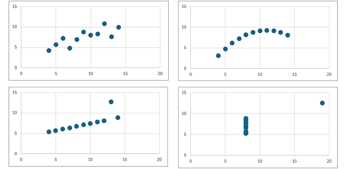
ome actuaries will be familiar with Anscombe’s quartet (Figure 1), created by Francis Anscombe in 1973.

The quartet shows four datasets, all of which have the same correlation between two variables. The graphic makes two important points:

Actuaries often make use of simulation models that include dependence among different variables. This may be, for example, multiple lines of business within a reinsurance treaty. It could also be part of an enterprise risk management (ERM) model concerned with the “tail risk” related to surplus adequacy.

An “Actuarial quartet” is proposed in Figure 2 to illustrate some different dependence structures common within actuarial applications. As with Anscombe’s quartet, all four have the same correlation between two random variables but with different dependence structures.

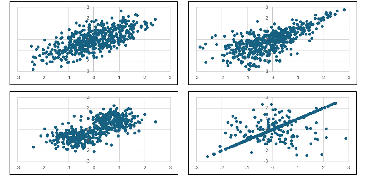
The upper left corner shows the correlation from a bivariate normal distribution. This can be generated from a Gaussian copula¹ and has the advantage of being easy to explain and expand to higher dimensions.

The Gaussian copula works well when we are working with the center or middle of the distribution. It is very useful for evaluating contract features such as sliding-scale commissions that vary close to the expected loss amounts. It is less useful when evaluating the “tail” of the distribution because the variables become effectively independent at the extremes.²

The upper right corner shows a relationship with heavy right-tail dependence. This can be generated from a few methods, with the Gumbel copula being a popular choice. This dependence structure is more useful in ERM or when evaluating out-of-the-money contract features such as stop-loss treaties.

The right-tail dependence is appropriate for cases where we believe everything can go wrong at once. An example might be extreme inflation changes or soft market cycle movement, affecting multiple lines of business simultaneously. It can be thought of as applying a skewed “mixing parameter” to otherwise independent random variables.

The lower left corner shows a relationship between clustered datasets. This is the type of dependence that could be generated in scenario testing for discrete events. We might think of political risks or war risks in this case. The simulation first decides the effect of the scenario on each variable, but within each scenario, the random variables are treated as independent.

The lower right corner shows one additional simulation structure that is common in modeling when we want the total correlation coefficient to match a selected value. If ρ=0.25, then 25% of the simulations assume perfect correlation between the variables, and the remaining 75% of the simulations assume independence. It is not so easy to describe business reasons for this structure, but it is an easy form to use as a benchmark, and it does create strong tail dependence.

As with Anscombe’s quartet, all the dependence structures in the Actuarial quartet have the same correlation coefficients and will therefore produce the same variance (and standard deviation) for the portfolio. But the choice of dependence structure will affect the shape of the portfolio aggregate distribution and the view of the tail risk. The visualization can help make sure that the tail risk reflects the characteristics of the business.